1 Pen-Tung Sah Institute of Micro-Nano Science and Technology, Xiamen University, Xiamen, 361102, China
2 School of Aerospace Engineering, Xiamen University, Xiamen, 361102, China
Corresponding author: wsj@xmu.edu.cn
|
Article Type Access License Received Revised Accepted Published Online Copyright |
Abstract. With the rapid advancement of artificial intelligence (AI) in industrial applications, this paper proposes a novel intelligent optimization method based on a hybrid data-model-driven approach to address traditional challenges in loader excavation trajectory optimization, including high data acquisition costs and computational complexity. First, a kinematic model of the loader working mechanism is established using the Denavit-Hartenberg (D-H) method to enable workspace mapping. Subsequently, an EDEM-RecurDyn co-simulation platform is developed to efficiently generate training datasets. Then, a linear trajectory ensuring the required excavation volume is then planned to define the end-effector pose constraints. The core contribution lies in the deep integration of physics-based modeling and data-driven intelligence. Specifically, an AI-based prediction model is developed to evaluate trajectory performance, and a corresponding fitness function is formulated. The IVY optimization algorithm is then employed for efficient autonomous optimization, with the optimal trajectory generated via spline fitting. Experimental results demonstrate that, compared with conventional metaheuristic algorithms, the proposed method improves convergence speed by approximately 88% and fitness value by approximately 26%. This research overcomes the limitations of purely data-driven or model-driven approaches, providing an efficient and cost-effective solution for intelligent construction machinery operation, and demonstrates the potential of AI technology in industrial trajectory optimization. |
Keywords: Data-model fusion; Excavation trajectory; Trajectory optimization; IVY algorithm; AI-based prediction
Key Takeaways
- Hybrid data–model loop pairs physics fidelity with AI speed.
- IVY optimizer accelerates convergence and improves fitness.
- Co-simulation + surrogate reduces data cost while retaining accuracy.
1. Introduction
Driven by the deep integration and advancement of Internet of Things (IoT), intelligent sensing, and artificial intelligence (AI) technologies [1-3], the industrial sector is currently undergoing a wave of innovation centered on intelligent driving. In this context, the construction machinery industry is accelerating its transformation and upgrading towards intelligence and autonomy [4], thereby promoting the industry's transition to an efficient, low-carbon, and intelligent construction model.
As a typical representative of earthmoving machinery, the loader is primarily used for excavation, transportation, and material dumping, undertaking critical tasks in scenarios such as mining, construction, and emergency rescue operations. During the excavation phase, the loader bucket continuously interacts with the ground and materials. Due to the involvement of highly nonlinear dynamics, time-varying material properties, and complex contact mechanics, coupled with demands for high efficiency, a high bucket fill rate, and low energy consumption, this phase is considered a bottleneck that constrains the overall improvement of operational performance. Thus, planning an intelligent excavation trajectory that comprehensively optimizes multiple performance indicators prior to the digging operation represents a core challenge in achieving safe, energy-efficient, and highly productive unmanned operations for loaders.
Currently, research on loader trajectory planning is predominantly focused on the vehicle travel phase, while studies specifically on the excavation phase remain relatively limited and are still in the exploratory stage. Existing excavation trajectory planning methods have not yet fully met the requirements of practical engineering applications. From the perspective of existing research practices, most methods tend to focus on optimizing a single performance indicator, either maximizing operational efficiency or only focusing on reducing energy consumption, lacking systematic trade-offs and collaborative optimization among bucket fill rate, energy consumption, and operation time, making it difficult to adapt to multi-objective operational requirements under complex working conditions. Meanwhile, existing methods either over-rely on physical modeling and ignore the actual operational laws in data, or simply rely on data-driven approaches without theoretical mechanism support, failing to achieve deep integration of physical mechanisms and data intelligence, resulting in difficulties in balancing the accuracy, applicability, and stability of trajectory optimization.
In summary, existing research still presents notable limitations: most optimization methods target relatively singular objectives, lacking systematic trade-offs among bucket fill rate, energy consumption, and time. Furthermore, the modeling and optimization processes fail to achieve deep integration of physical mechanisms with data intelligence.
To address these gaps, this paper, based on engineering intelligence and system innovation, proposes a hybrid-driven optimization method for loader excavation trajectory that deeply integrates physical mechanisms with data intelligence. This method establishes a closed-loop framework consisting of kinematic modeling, co-simulation data generation, AI-based performance prediction, and intelligent optimization. Through the three-level synergy among mechanism, data, and algorithm, the proposed method achieves a balance among accuracy, efficiency, and engineering applicability in trajectory optimization. The main innovations of this work are as follows: (1) construction of an integrated EDEM–RecurDyn simulation platform coupled with an AI-based prediction model for accurate and efficient trajectory performance estimation; (2) introduction of the IVY algorithm for intelligent optimization, achieving rapid and high-quality trajectory generation; (3) establishment of a bidirectional data–model-driven optimization system validated through both simulations and real-world experiments.
2. Related Work
First, Model-driven Trajectory Planning and Optimization Methods This category of methods carries out planning based on mathematical, physical, and similarity models. Frank B et al. [5] developed a dynamic programming framework that leverages optimal control theory to enhance fuel economy by optimizing the speed, bucket lift position, and tilt position of a wheel loader. Yao J et al. [6] developed a control-oriented model for bucket loading operations, transformed it into an optimal control problem with physical constraints, and employed the OpenOCL solver for numerical solution. Simulations indicated that this method significantly improves energy efficiency. Zhang T et al. [7] utilized the Lagrangian method to construct a mechanical-ore coupled dynamic model for electric shovels and, combined with a multi-objective trajectory optimization approach using the pseudospectral method, obtained optimal digging trajectories. Chen Y et al. [8] established a mathematical model for loader fuel consumption during excavation using Support Vector Machines and optimized the excavation trajectory by integrating an improved Particle Swarm Optimization algorithm, achieving energy saving and consumption reduction. Timofeev I P et al. [9] employed techniques such as vector algebra, second-order central difference, and triangulation to develop a kinematic model for the loader bucket, optimizing the excavation trajectory for bulk materials. Tan X et al. [10] proposed a hybrid method combining Particle Swarm Optimization and Reinforcement Learning, enabling continuous trajectory planning and optimization for excavators during trenching operations.
Second, Data-driven Trajectory Planning and Optimization Methods Huai Z et al. [11] conducted actual excavation tests using a loader to obtain data at different digging depths. By comparing various methods, they found that the piecewise cubic Hermite interpolation regression method offered the best prediction accuracy, and based on this, they identified a trajectory that achieves a high bucket fill rate. Zhou T et al. [12] acquired loader operational performance parameters at various excavation depths and optimized the excavation trajectory using a parabolic interpolation method calibrated with experimental data, thereby reducing operational energy consumption. Zhang T et al. [13] proposed a rotational speed-based data-driven approach, utilizing actual excavation data from unmanned mining excavators to dynamically predict resistance. The trajectory was then optimized via a deep learning algorithm and ultimately validated on a scaled prototype. Dadhich S et al. [14] established a linear regression model based on expert operational data to predict bucket lift and tilt actions and employed a reinforcement learning method to optimize parameters, achieving more efficient bucket loading trajectory planning.
Third, Hybrid Data-model Driven Trajectory Planning and Optimization Methods Li S et al. [15] employed a joint modeling approach integrating feedforward neural networks and physics-informed encoding optimization. Compared to traditional trajectory planning based solely on numerical optimization, this method enables more efficient, energy-saving, and real-time feasible excavation trajectory planning. Meng Y et al. [16] established a resistance model for the loader bucket based on Coulomb's theory and optimized the bucket trajectory with the principle of minimum energy consumption, which was subsequently validated through simulations in EDEM software. Yu X et al. [17] used the Kriging method to build an agent model describing the relationship between the loader's snow-removal trajectory and its efficiency. Combined with RecurDyn-EDEM co-simulation, they obtained optimal snow-removal trajectories for different working conditions. Zhao Q et al. [18] used Doppler Generative Adversarial Network to augment continuous excavation data to obtain enriched data, and then combined it with reinforcement learning to achieve automatic trajectory planning.
A comprehensive analysis of the above studies shows that model-driven methods provide solid theoretical foundations and can deliver mathematically optimal solutions. However, they suffer from high computational complexity and often fail to fully account for the environmental randomness and operational complexities inherent in earthmoving machinery, resulting in significant discrepancies between theoretical analyses, simulation models, and actual operations, which makes it difficult to achieve the desired outcomes in practical applications. Data-driven methods can adapt to nonlinear systems and reflect patterns observed in real-world working conditions, yet they come with high data acquisition costs, rely heavily on data quality, and exhibit weak interpretability. In comparison, the hybrid data-model driven approach effectively balances theoretical precision with engineering practicality. By integrating prior knowledge with experimental data, it reduces reliance on extensive datasets and lowers modeling costs, demonstrating significant advantages in complex trajectory planning for unmanned construction machinery. Nevertheless, existing hybrid-driven methods still fail to address the issues of multi-objective collaborative optimization and deep integration of mechanisms and data. The hybrid-driven optimization method proposed in this paper precisely compensates for the above shortcomings — through a three-level collaborative architecture of mechanism, data, and algorithm, it achieves deep integration of physical mechanisms and data intelligence. Meanwhile, relying on the IVY algorithm and co-simulation prediction model, it can perform multi-objective collaborative optimization of bucket fill rate, energy consumption, and operation time, balancing the accuracy, efficiency, and engineering applicability of trajectory optimization, and providing more reliable technical support for unmanned excavation operations of loaders.
Inspired by the latest similar method [15] in this field, that study adopts a technical route of “optimization algorithm generating samples, feedforward neural network rapidly predicting trajectories, and physics-informed encoding optimization for refinement”. It centers on data prediction, with the physical model serving as a supplementary correction tool in the later stage, thereby fully leveraging the advantages of a hybrid model. The hybrid-driven optimization method proposed in this paper innovatively establishes a closed-loop system of “physical mechanism modeling, co-simulation generating high-fidelity data, AI performance prediction, and intelligent algorithm for trajectory optimization”. It uses a physical model to construct the overall optimization framework, employs data intelligence to enhance prediction accuracy, and relies on an intelligent algorithm to accomplish trajectory optimization, truly achieving a bidirectional and deep integration of physical mechanisms and data intelligence. Moreover, by leveraging the IVY optimization algorithm and the co-simulation-based prediction model, it realizes multi-objective collaborative optimization covering bucket fill factor, energy consumption, and operation time, striking a balance among accuracy, efficiency, and engineering applicability in trajectory optimization, thus providing more reliable technical support for unmanned excavation operations of loaders.
3. Method
3.1. Overall Framework
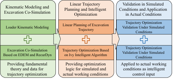
To achieve comprehensive and intelligent optimization of the loader excavation trajectory, this study proposes a systematic methodological framework driven by hybrid data-model integration. As illustrated in Fig. 1, the framework follows the technical pathway of "physical modeling → data generation → intelligent optimization → trajectory generation". It seamlessly integrates kinematic mechanisms, multiphysics simulation, and artificial intelligence algorithms to establish an efficient and cost-effective optimization platform.
3.2. Kinematic Modeling of the Loader
To achieve accurate description and control of the bucket-end trajectory, it is essential to establish the mapping relationships among the driving space, joint space, and task space of the loader's working mechanism. This provides the theoretical foundation for subsequent intelligent trajectory optimization. This section focuses on the inverted six-linkage working mechanism of a 1:4 scaled prototype, which is designed based on the XG958i loader. By simplifying its complex three-dimensional motion to a two-dimensional planar motion, the kinematic model is established using the Denavit-Hartenberg (D-H) method.
3.2.1. Kinematic Analysis of the Working Mechanism
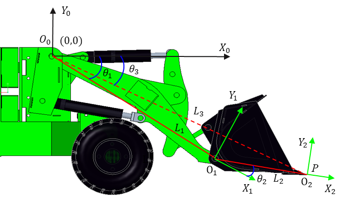
During material excavation, the coordinated motion of the entire machine's travel movement along with the extension and retraction of the lift cylinder and bucket tilt cylinder controls the bucket's position and orientation to perform the digging operation. Given that the working mechanism exhibits symmetrical planar motion during excavation, it is simplified as a two-dimensional inverted six-link mechanism. A Cartesian coordinate system is established with the hinge point O0 between the boom and the front frame as the origin, the forward direction of the entire machine as the positive X-axis, and the vertical upward direction perpendicular to the ground as the positive Y-axis, as illustrated in Fig. 2.

3.2.2. Transformation from Task Space to Joint Space
Based on the D-H method, the homogeneous transformation matrix between adjacent coordinate systems is established, as shown in (1). By linking the transformation matrices between adjacent coordinate systems, the overall transformation relationship from the initial coordinate system to the end-effector coordinate system is established, yielding the total transformation matrix that describes the motion of the entire system, as presented in (2).
| \[{}_{i}^{\,i - 1}T = T_{Z_{i - 1}}(\theta_{i}) T_{Z_{i - 1}}(d_{i}) T_{X_{i}}(a_{i}) T_{X_{i}}(\alpha_{i}) = \begin{bmatrix} \cos\theta_{i} & -\sin\theta_{i}\cos\alpha_{i} & \sin\theta_{i}\sin\alpha_{i} & a_{i}\cos\theta_{i} \\ \sin\theta_{i} & \cos\theta_{i}\cos\alpha_{i} & -\cos\theta_{i}\sin\alpha_{i} & a_{i}\sin\theta_{i} \\ 0 & \sin\alpha_{i} & \cos\alpha_{i} & d_{i} \\ 0 & 0 & 0 & 1 \end{bmatrix}\] | (1) |
In the equation, \(\theta_{i}\) represents the angle between \(X_{i - 1}\) and \(X_{i}\) as viewed from the \(Z_{i - 1}\) direction (positive for right-handed rotation);\(\alpha_{i}\) represents the angle between \(Z_{i - 1}\) and \(Z_{i}\) as viewed from the \(X_{i}\) direction (positive for right-handed rotation);\(d_{i}\) represents the distance between \(X_{i - 1}\) and \(X_{i}\) along the \(Z_{i - 1}\) direction (positive when aligned with \(Z_{i - 1}\));\(a_{i}\) represents the distance between \(Z_{i - 1}\) and \(Z_{i}\) along the \(X_{i}\) direction (positive when aligned with \(X_{i}\))
| \[{}_{n}^{0}\mathbf{T} = {}_{1}^{0}\mathbf{T}\,{}_{2}^{1}\mathbf{T}\,{}_{3}^{2}\mathbf{T}\cdots {}_{n - 1}^{n - 2}\mathbf{T}\,{}_{n}^{n - 1}\mathbf{T}\] | (2) |
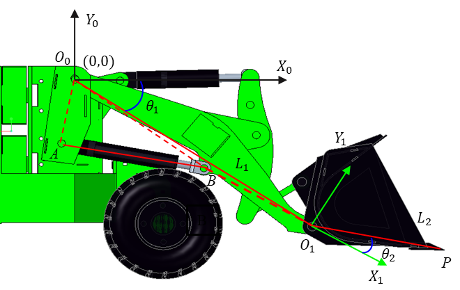
Simplify the working mechanism model of the loader and establish the D-H coordinates as shown in Fig. 3. Take hinge point \(O_{0}\) between the boom and the front frame as the origin of the initial coordinate system, hinge point \(O_{1}\) between the boom and the bucket as the origin of the second coordinate system, and the bucket tooth tip \(O_{2}\) as the origin of the end-effector coordinate system. Furthermore, the common perpendicular between axis \(Z_{0}\) and axis \(Z_{1}\) is defined as line \(O_{0}O_{1}\), whose direction corresponds to the positive direction of the \(X_{1}\)-axis. The direction of the \(Y_{1}\)-axis is determined using the right-hand rule. Similarly, the directions of \(X_{2}\) and \(Y_{2}\) can be established following the same principle.
Within the established D-H coordinate system above, the pose of the loader's inverted six-link mechanism is determined by the following four parameters:\(\alpha_{i}\)、\(a_{i}\)、\(\theta_{i}\)、\(d_{i}\), as listed in TABLE I (where Joint 1 and Joint 2 correspond to the boom joint and bucket joint, respectively). Substituting these parameters into (1) yields the homogeneous transformation matrix of the bucket tooth tip relative to the initial coordinate system, as shown in (3).
TABLE I
Joint Parameter Values
| Joint i | \[\theta_{i}\] | \[d_{i}\] | \[a_{i}\] | \[\alpha_{i}\] |
| 1 | \[\theta_{1}\] | 0 | \[L_{1}\] | 0 |
| 2 | \[\theta_{2}\] | 0 | \[L_{2}\] | 0 |
| \[\begin{bmatrix} \cos(\theta_{1} + \theta_{2}) & -\sin(\theta_{1} + \theta_{2}) & 0 & L_{2}\cos(\theta_{1} + \theta_{2}) + L_{1}\cos\theta_{1} \\ \sin(\theta_{1} + \theta_{2}) & \cos(\theta_{1} + \theta_{2}) & 0 & L_{2}\sin(\theta_{1} + \theta_{2}) + L_{1}\sin\theta_{1} \\ 0 & 0 & 1 & 0 \\ 0 & 0 & 0 & 1 \end{bmatrix}\] | (3) |
Assume the coordinates of the bucket endpoint in the initial coordinate system are (\(P_{x}\),\(P_{y}\),0), then:
| \[\left\{ \begin{aligned} P_{x} &= L_{2}\cos(\theta_{1} + \theta_{2}) + L_{1}\cos\theta_{1} \\ P_{y} &= L_{2}\sin(\theta_{1} + \theta_{2}) + L_{1}\sin\theta_{1} \\ P_{z} &= 0 \end{aligned} \right.\] | (4) |
Considering the coordinated action of vehicle displacement s during excavation, and given that the excavation trajectory consists of multiple (\(X\),\(\ Y\)) points, the inverse kinematic solution can be derived by incorporating (4). This leads to the inverse kinematic model that transforms the task space of the loader into the joint space, as expressed in (5) to (7).
| \[\theta_{1} = \frac{{(X - s)}^{2} + Y^{2} + {L_{1}}^{2} - {L_{2}}^{2}}{2L_{1}\sqrt{{(X - s)}^{2} + Y^{2}}}\] | (5) |
| \[\theta_{2} = \frac{\sqrt{{(X - s)}^{2} + Y^{2}}sin(\theta_{3} - \theta_{1})}{L_{2}}\] | (6) |
| \[\theta_{3}\ = \ \tan^{- 1}\frac{Y}{X - s}\ \ \] | (7) |
In the equations, \(\theta_{1} > 0\) corresponds to boom lifting, while \(\theta_{1} < 0\) corresponds to boom lowering; \(\theta_{2} > 0\) corresponds to bucket upward rotation, while \(\theta_{2} < 0\) corresponds to bucket downward rotation; \(\theta_{3}\) represents the angle between the line connecting point P to point \(O_{0}\) and the X-axis of the initial coordinate system.
3.2.3. Transformation from Joint Space to Actuator Space
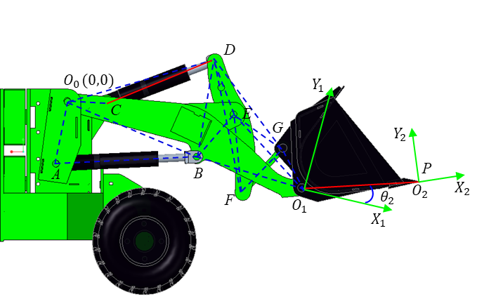
Based on the structure of the working mechanism, a geometric diagram of the boom is illustrated in Fig. 4. By combining the cosine theorem of △\({AO}_{0}B\) from (8) and the geometric relationship from (9), the relationship between \(\theta_{1}\) and\({\ L}_{AB}\) is derived as shown in (10).
| \[\angle{AO}_{0}B = \arccos^{\ }\frac{L_{O_{0}B}^{2} + L_{O_{0}A}^{2} - L_{AB}^{2}}{2{\cdot L}_{O_{0}B} \cdot L_{O_{0}A}}\] | (8) |
| \[\angle{AO}_{0}B = \angle{AO}_{0}X_{0} - \angle BO_{0}O_{1} - \theta_{1}\] | (9) |
| \[L_{AB} = \sqrt{L_{O_{0}B}^{2} + L_{O_{0}A}^{2} - 2L_{O_{0}B} \cdot L_{O_{0}A}{\cdot cos(\angle{AO}_{0}X_{0} - \angle BO_{0}O_{1} - \theta_{1})}^{\ }}\] | (10) |
A schematic diagram of the bucket-tilting geometric relationship is illustrated in Fig. 5. Through the sine theorem, cosine theorem, and geometric relationships concerning △\({EO}_{1}B\)、△\({EO}_{1}G\)、△\(EFG\)、△\(DFG\)、△\(DEG\)、△\(BDE\)、△\(BO_{0}D\)、△\(AO_{0}D\) and △\(CO_{0}D\), as expressed in (11) to (25), the mapping relationship between \(\theta_{2}\) and\({\ L}_{CD}\) is obtained.
| \[\angle{EO}_{1}G = 180{^\circ} - \theta_{2} - \angle{O_{0}O}_{1}E - \angle{{GO}_{1}O}_{2}\] | (11) |
| \[L_{EG} = \sqrt{L_{EO_{1}}^{2} + L_{GO_{1}}^{2} - 2L_{EO_{1}} \cdot L_{{GO}_{1}}{\cdot cos\angle{EO}_{1}G}^{\ }}\] | (12) |
| \[\angle{GEO}_{1} = arcsin\frac{L_{{GO}_{1}} \cdot sin\angle{EO}_{1}G}{L_{EG}}\ \] | (13) |
| \[\angle EFG = arccos\frac{L_{EF}^{2} + L_{FG}^{2} - L_{EG}^{2}}{2{\cdot L}_{EF} \cdot L_{FG}}\] | (14) |
| \[L_{DG} = \sqrt{L_{DF}^{2} + L_{FG}^{2} - 2L_{DF} \cdot L_{FG}{\cdot cos\angle DFG}^{\ }}\] | (15) |
| \[\angle DFG = \angle DFE + \angle EFG\ \] | (16) |
| \[\angle DEG = arccos\frac{L_{DE}^{2} + L_{EG}^{2} - L_{DG}^{2}}{2{\cdot L}_{DE} \cdot L_{EG}}\] | (17) |
| \[L_{BD} = \sqrt{L_{DE}^{2} + L_{BE}^{2} - 2L_{DE} \cdot L_{BE}{\cdot cos\angle BED}^{\ }}\] | (18) |
| \[\angle BED = 360{^\circ} - \angle BEO_{1} - \angle O_{1}EG - \angle DEG\ \] | (19) |
| \[\angle EBD = arcsin\frac{L_{DE} \cdot sin\angle BED}{L_{BD}}\] | (20) |
| \[\angle O_{0}BD = 360{^\circ} - \angle O_{0}BO_{1} - \angle O_{1}BE - \angle EBD\ \ \ \] | (21) |
| \[L_{O_{0}D} = \sqrt{L_{O_{0}B}^{2} + L_{BD}^{2} - 2L_{O_{0}B} \cdot L_{BD}{\cdot cos\angle O_{0}BD}^{\ }}\] | (22) |
| \[\angle BO_{0}D = arcsin\frac{L_{BD}sin\angle O_{0}BD}{L_{O_{0}D}}\] | (23) |
| \[\angle CO_{0}D = \angle BO_{0}D + \angle AO_{0}B - \angle AO_{0}C\] | (24) |
| \[L_{CD} = \sqrt{L_{CO_{0}}^{2} + L_{O_{0}D}^{2} - 2L_{{CO}_{0}} \cdot L_{O_{0}D}{\cdot cos\angle{CO}_{0}D}^{\ }}\] | (25) |
In summary, the relationships between the lengths of the lift cylinder \(L_{AB}\) and the bucket tilt cylinder \(L_{CD}\) as functions of the joint rotation angles \(\theta_{1}\) and \(\theta_{2}\) can be established, while all other working mechanism parameters are known design values.
3.3. EDEM-RecurDyn Co-Simulation for Excavation
Discrete Element Method–Multibody Dynamics (DEM-MBD) co-simulation can precisely reveal the coupling effects between component motion and soil loads and has been widely adopted for analyzing soil–machine interaction mechanics. Given the extended time and high costs associated with physical experimental data acquisition, and considering that existing studies [19-21] have demonstrated the effectiveness of EDEM-RecurDyn coupled simulation in replicating the loader excavation process, this research establishes a co-simulation platform to generate high-quality datasets. This platform provides essential data support for the subsequent construction of an intelligent trajectory optimization model.
3.3.1. EDEM-Based Material Modeling
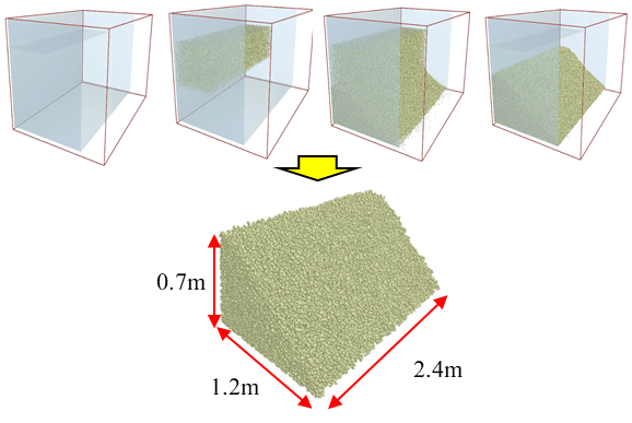
This study employs the Discrete Element Method within EDEM to construct a crushed stone material model, aiming to accurately simulate the interaction behavior between the material and the bucket. The modeling process is as follows: Firstly, the particle shape and particle size distribution are determined. Three particle shapes are mixed in equal mass proportions, and the particle size distribution, based on standard sieve analysis, is set as 10 mm (40%), 15 mm (30%), 20 mm (20%), and 25 mm (10%). Secondly, referring to relevant co-simulation literature [19], the intrinsic parameters and contact parameters for the material and the bucket are configured. Finally, particles are generated using a particle factory, with the generation area bounded to match the bucket width to reduce computational costs. To replicate the diversity of material piles in real working conditions, multiple material piles with different angles of repose are generated. This paper takes a typical working condition as an example: the generated material pile has a base dimension of 2.4 m × 1.2 m, a top height of 0.7 m, and an angle of repose of 34°, as shown in Fig. 6.
3.3.2. RecurDyn-Based Multibody Dynamics Modeling
This study develops a multibody dynamics model of the loader in RecurDyn to simulate the motion and force characteristics of its components. Constraints are defined, as listed in TABLE II, to enable motion transfer between the parts. Furthermore, to realize the excavation process, drive functions need to be configured in RecurDyn.
TABLE II
Constraint Relationships of the Complete Vehicle
| Joint Type | Constraint |
| Contact | Wheel – Ground |
| Revolute | Drive Wheel–Frame |
| Revolute | Link – Bucket |
| Revolute | Lift Cylinder Rod – Boom |
| Revolute | Boom – Front Frame |
| Revolute | Lift Cylinder – Front Frame |
| Revolute | Link – Rocker Arm |
| Revolute | Rocker Arm – Bucket-tilting Cylinder Rod |
| Revolute | Bucket-tilting Cylinder – Front Frame |
| Translational | Lift Cylinder – Lift Cylinder Rod |
| Translational | Bucket-tilting Cylinder – Bucket-tilting Cylinder Rod |
3.3.3. Co-Simulation Setup and Implementation
After completing the multibody dynamics model and the discrete element material model, a bidirectional coupled co-simulation is conducted. The WALL file exported from RecurDyn is imported into EDEM, enabling real-time transfer of mechanical system parameters to the discrete element model. Simultaneously, EDEM feeds back granular dynamic loads to RecurDyn, forming a closed-loop mechanical interaction. By adjusting the drive functions to simulate various excavation depths and speed conditions, the simulation data is enriched, thereby enhancing the engineering representativeness of the dataset.
To accurately characterize the morphology of the material pile and support subsequent intelligent trajectory planning, a polynomial surface fitting method from previous work [19] is adopted for three-dimensional reconstruction of the material surface, obtaining key features: (1) Extract the height of the material surface corresponding to the bucket tip trajectory as input for operational resistance prediction; (2) The material's angle of repose is determined by fitting the linear term, providing a basis for initial linear trajectory planning; (3) Based on the fitted surface of the material pile, the excavation volume is estimated.
After the co-simulation, the time-series 3D coordinate data of material particles exported from EDEM are extracted and preprocessed to obtain the particle coordinate sets for all time steps. A polynomial fitting surface equation is established as shown in (26). By substituting the bucket tip trajectory’s X- and Y-axis data, derived from forward kinematics, into the equation, the corresponding material surface height at each trajectory point can be calculated.
| \[f(x,y) = a_{0} + a_{1}x + \cdots + a_{m}x^{m} + b_{0} + b_{1}y + \cdots + b_{n}y^{n}\] | (26) |
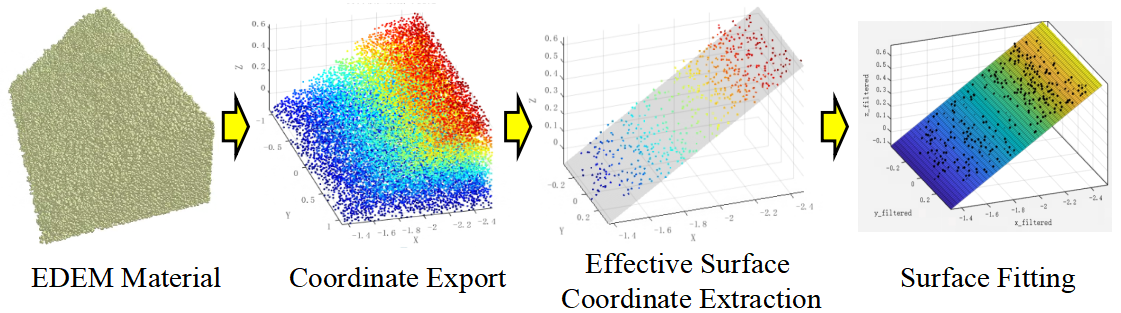
By retaining the constant term and the linear term of the aforementioned surface equation, the material's angle of repose is estimated through linear term fitting. Specifically, when setting y equal to 0, the formula reduces to a straight-line equation in the X-Z plane. The slope of this line is calculated to derive the angle between the material slope and the ground. Limited by the bucket width, only the material surface within the bucket width range needs to be considered during fitting. The specific steps are illustrated in Fig. 7. Following the above procedure, the material's angle of repose is ultimately determined to be 34°, providing essential information on material slope for linear trajectory planning.
3.4. Excavation Trajectory Planning
The preceding sections completed material modeling and surface feature extraction through EDEM-RecurDyn co-simulation. Based on engineering operational requirements and material characteristics, this section first analyzes the suitability of typical excavation methods. It then establishes initial constraint boundaries through linear trajectory planning, thereby delineating an effective search space for subsequent intelligent trajectory optimization and enhancing both optimization efficiency and engineering adaptability.
3.4.1. Analysis of Excavation Methods
The mainstream excavation methods for current loaders include one-pass digging, segmented digging, and slice digging. This study selects one-pass digging and slice digging as the planning targets for excavation strategies, based on the following rationale for their suitability: (1) From the perspective of operational feasibility, the one-pass digging method features a discrete and intuitive action sequence, which is easily translatable into automated control commands, making it well-suited for the transition from manual to intelligent automated operations. (2) In terms of energy efficiency, Chen Y et al. [8] have confirmed that the slice digging method reduces operational resistance through a layered cutting mechanism, resulting in a smooth excavation process and ensuring a high bucket fill rate. (3) Regarding adaptability to working conditions, one-pass digging and slice digging form a complementary technical pair: the former is suitable for the rapid handling of loose materials, while the latter is applicable to scenarios involving dense materials. This combination can cover typical working conditions, laying a foundation for constructing a universal automatic excavation trajectory optimization framework.
3.4.2. Linear Trajectory Planning for Excavation
In the world coordinate system, excavation trajectories can be categorized into linear trajectories and curved trajectories. Filla et al. [22] generated 800 sets of trajectories and conducted comparisons, demonstrating the advantages of linear excavation trajectories. Although constrained by the kinematic limitations of the loader’s linkage mechanism, which prevents the bucket from following a strictly linear trajectory, and while linear trajectories tend to induce abrupt variations in joint-space curves that pose challenges for control, the concept of linear planning can still be utilized to rapidly estimate excavation volume. This approach helps clarify the range of motion required for the working mechanism to meet excavation volume requirements, thereby narrowing the search space for subsequent intelligent trajectory optimization and improving overall efficiency.
From a two-dimensional planar perspective, the surface of the material pile can be approximated as a straight line with a fixed slope. The area enclosed by the excavation trajectory (blue polyline) and the material surface (red straight line) constitutes the excavation area S, as shown in Fig. 8. Combined with the bucket width, the excavation volume can be derived as expressed in (27).
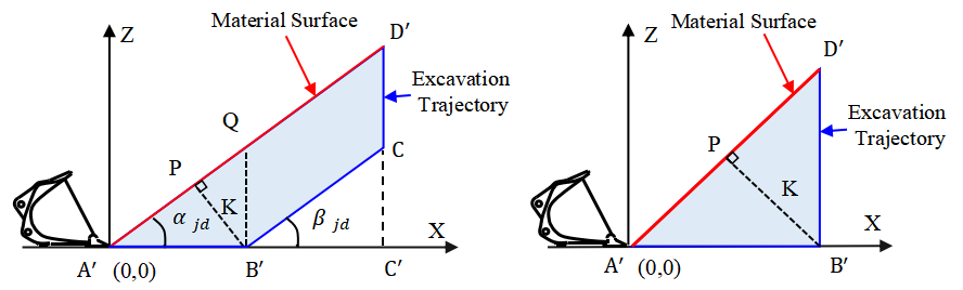
(a)Slice Digging (b)One-pass Digging
Fig. 8. Schematic Diagram of Linear Trajectory Planning
| \[V = B \times S = \frac{BK}{2}(L_{A'D'} + L_{B'C})\] | (27) |
In the equation, V represents the volume of material that can be excavated by the trajectory; B represents the bucket width; K represents the normal distance between the linear excavation trajectory and the material pile surface; and \(\alpha_{jd}\) represents the angle of repose of the material pile.
Drawing on the research by Chen Y et al. [8], in the linear slice excavation method, when the inclination angle \(\beta_{jd}\) of the straight-line segment \(B'C\) equals the angle of repose \(\alpha_{jd}\) of the material pile, it is referred to as a parallel excavation trajectory, which results in lower operational resistance. Combining this with the inference by Chen Yanhui et al. [23], the trajectory equation of the bucket tip can be defined as (28):
| \[\left\{ \begin{aligned} L_{A'B'} &= \frac{K}{\sin\alpha_{jd}} \\ L_{B'C} &= \frac{G}{K\rho(1 - N)B} - \frac{K}{\sin(2\alpha_{jd})} \\ L_{CD'} &= \frac{K}{\cos\alpha_{jd}} \end{aligned} \right.\] | (28) |
In the equation, G represents the rated bucket load capacity of the loader; \(\rho\) represents the material density; and N represents the material porosity. Since this study targets crushed stone as the material, \(\rho\) = 2600 kg/m³ and N = 39.9%.
Since the material density, porosity, angle of repose of the pile, bucket width, and bucket load capacity are all known parameters, the position of the bucket tip can be expressed as a function of K. By adjusting the value of K and substituting it into (28), an excavation trajectory that meets the target excavation volume can be planned. When K = \(L_{A'B'} \ast \sin\alpha_{jd}\), it represents one‑pass excavation. Since one‑pass excavation does not include the \(L_{B'C}\) segment, the term \(L_{B'C}\) in (27) must be set to zero when calculating the excavation area.
Based on the above analysis, this study proposes the following workflow for determining the motion range of the loader’s working mechanism: First, the material’s angle of repose and the actual bucket parameters are determined, and the variation range of K is defined. Then, the excavation volume is estimated using (27) and (28), with the volume constrained to 80%–110% of the rated bucket capacity, while also limiting the ranges of \(L_{A'B'}\) and \(L_{A'C'}\). Finally, candidate straight‑line trajectories are generated with a step size of 5 mm, resulting in a feasible range of K values that satisfy the conditions. Through kinematic transformation, the final feasible range of boom angles that meet the constraints can be derived, thereby providing variable bounds for subsequent trajectory optimization.
3.5. Optimization Objectives and Variables for Excavation Trajectory
Trajectory optimization serves as the core component for achieving intelligent excavation, requiring clear definition of optimization variables, quantitative formulation of objectives, and a fitness function. Building on the trajectory planning and co‑simulation data presented earlier, this section determines the optimization variables and objectives based on the engineering requirements of high efficiency, low energy consumption, and high bucket fill rate, thereby laying the groundwork for the subsequent application of the IVY intelligent optimization algorithm.
3.5.1. Optimization Variables
Unlike the "insert-lift-insert-lift" strategy of segmented digging methods, both single-pass digging and slice digging are realized through the continuous transitions of boom motion, bucket-tilting action, and vehicle displacement. Therefore, only the initial values, terminal values, and the duration of each phase for these three types of motion need to be planned. Analyzing the suitability for optimization across driving space, joint space, and task space reveals the following: optimization in the driving space is not directly linked to the bucket trajectory, making it prone to deviation and difficult to handle joint constraints, which results in poor adaptability. While task-space planning is intuitive, its inverse kinematic reconstruction may lead to multiple solutions or singularities. In contrast, the joint space, as the intermediate kinematic layer connecting the task space and the driving space, enables dual-trajectory tracking and enhances accuracy. Therefore, this study selects the joint space to conduct trajectory optimization.
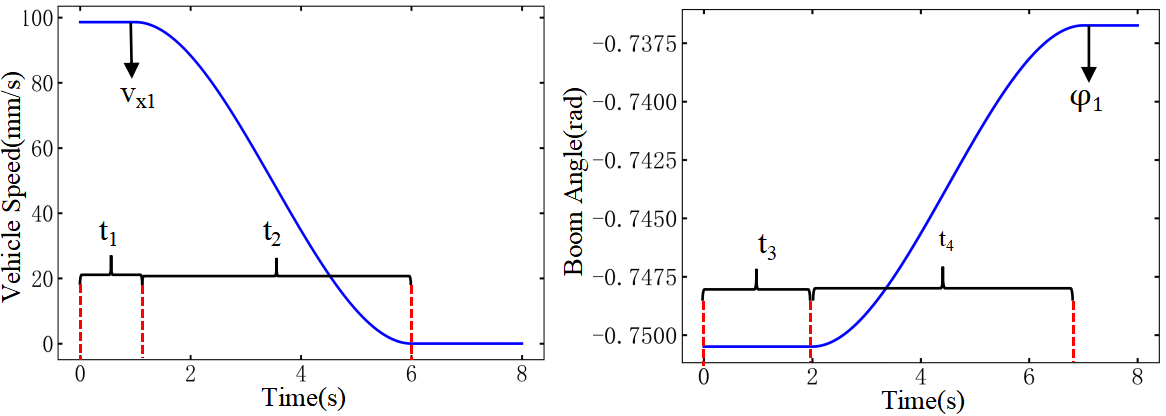
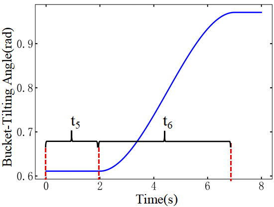
In the joint space, different excavation trajectories can be generated by adjusting the initial and final values of each variable as well as the timing of their changes. To prevent material spillage after the operation is completed, the bucket‑tilting cylinder rod must be fully extended, and the bucket‑tilting angle must reach its designed maximum value. Accordingly, the variables to be optimized are determined as follows: the duration \(t_{1}\) of the vehicle’s uniform forward phase, the duration \(t_{2}\) of the deceleration phase, the duration \(t_{3}\) of the boom static phase, the duration \(t_{4}\) of the boom lifting phase, the duration \(t_{5}\) of the bucket static phase, the duration \(t_{6}\) of the bucket‑tilting phase, the initial excavation speed \(v_{x1}\), and the final boom angle \(\varphi_{1}\), as illustrated in Fig. 9.
 |
|
| (a)Optimization Variables for the Vehicle Speed Curve | (b)Optimization Variables for the Boom Angle Curve |
 |
|
(c)Optimization Variables for The Bucket-Tilting Angle Curve |
|
Fig. 9. Schematic Diagram of Joint Space Variables
3.5.2. Excavation Volume Acquisition
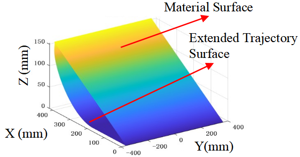
Unlike the linear trajectory planning in Section 2.4, which only required obtaining the angle of repose, the trajectory optimization stage must accurately estimate the excavation volume by integrating the current material pile morphology with the pre‑planned trajectory, thereby serving as one of the optimization objectives for determining the optimal trajectory. After approximating the material surface equation through polynomial fitting, the Alpha‑shape algorithm from prior work [24] is adopted to compute the material volume envelope. The specific calculation procedure is as follows:First, based on the linear planning results, key trajectory points (start and end points) are identified to ensure all trajectory points lie below the material surface, forming a valid calculation region. Second, the trajectory points are extended along the Y‑axis to form a trajectory surface, and the coordinate systems of the trajectory surface and the fitted material surface equation are aligned. Finally, the Alpha‑shape envelope calculation is performed in combination with the fitted polynomial of the material surface. The schematic diagram of the envelope is shown in Fig. 10.
3.5.3. Excavation Time Acquisition
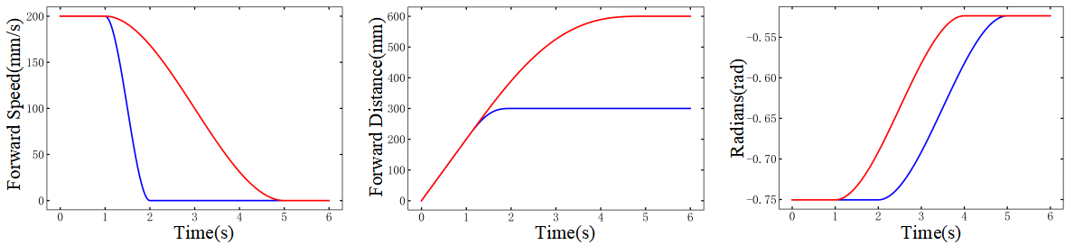
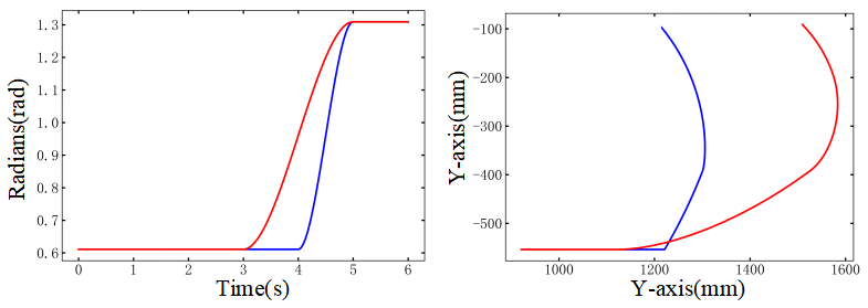
Based on the D-H method analysis in Section 2.2, different bucket-tip trajectories can be generated by adjusting the time parameters of the boom rotation angle, bucket-tilting angle, and vehicle speed curves. As shown in Fig. 11, different configurations of vehicle speed timing parameters (a) lead to variations in the final displacement (b). Similarly, different starting times for changes in the bucket-tilting and boom angle curves (c, d) ultimately result in distinct bucket trajectories (e), confirming the decisive role of time parameters on the trajectory. The excavation time is quantified as follows: by comparing the durations of planned motion phases in each joint space, the longest duration is selected as the excavation time metric, ensuring coverage of the entire operation process.
 |
|
| (a)Vehicle Speed Variation Curve | (b)Vehicle Displacement Variation Curve |
|
 |
| (c)Boom Angle Variation Curve | (b)Bucket‑Tilting Angle Variation Curve |
|
|
(e)Bucket-Tip Trajectory Variation Curve |
|
Fig. 11. Variation curves of the task space under different time-parameter configurations in the joint space
3.5.4. Excavation Resistance Acquisition
The operating resistance of a loader is a key parameter in the transmission system, used to characterize energy consumption. Its magnitude is closely related to the working trajectory [25], making accurate prediction of operating resistance crucial for trajectory optimization. In practical operations, resistance can be predicted using signals such as pressure and displacement by inputting sensor data from the current moment to forecast resistance at future times. However, trajectory planning is a pre‑decision process and cannot utilize cylinder pressure data from actions that have not yet been executed. Therefore, only two types of predictable parameters, displacement and angle, are selected as modeling features.
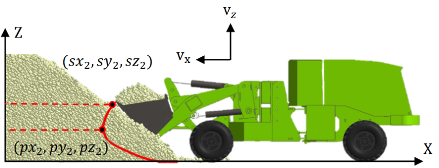
Thus, the input features for the trajectory‑based operating resistance prediction model developed in this study are: the time‑varying position information \((PX,PY,PZ)\) and velocity information \((VX,VY,VZ)\) of the loader bucket tip along the three coordinate directions of the excavation trajectory, together with the material surface information \((SX,SY,SZ)\). The output is the excavation resistance F. As \(PY\) and \(SY\), and \(PX\) and \(SX\) are numerically equivalent, as shown in Fig. 12, the input feature dimension is simplified to seven.
In the simulation environment, the three‑axis position and velocity information of the loader bucket tip are obtained via RecurDyn. However, when applied in real‑world scenarios, it is still necessary to rely on the loader kinematic model described in Section 2.2 of this paper. By inputting the planned joint‑space trajectory information, the actual bucket‑tip trajectory can be derived, and velocity information can then be obtained through time differentiation. Subsequently, given the material surface fitting equation \(Z = f(X,Y)\) and under the condition that the coordinate systems of the excavation trajectory information and the material surface fitting equation are unified, the position coordinates of the bucket tip at each time instant are substituted into the equation to obtain the corresponding material surface height. Finally, the information \(D_{track}\) for each excavation trajectory is obtained, expressed as follows:
| \(D_{track} = \lbrack T,PX,PY,PZ,VX,VY,VZ,SZ,F\rbrack\)=\(\left\lbrack \begin{matrix} t_{0} & px_{t_{0}} & p\text{y}_{t_{0}} & pz_{t_{0}} & \text{v}\text{x}_{t_{0}} & \text{v}\text{y}_{t_{0}} & \text{v}\text{z}_{t_{0}} & \text{s}\text{z}_{t_{0}} \\ t_{1} & px_{t_{1}} & p\text{y}_{t_{1}} & p\text{z}_{t_{1}} & \text{v}\text{x}_{t_{1}} & \text{v}\text{y}_{t_{1}} & \text{v}\text{z}_{t_{1}} & \text{s}\text{z}_{t_{1}} \\ \vdots & \vdots & \vdots & \vdots & \vdots & \vdots & \vdots & \vdots \\ t_{\text{n-1}} & px_{t_{\text{n-1}}} & p\text{y}_{t_{\text{n-1}}} & p\text{z}_{t_{\text{n-1}}} & \text{v}\text{x}_{t_{\text{n-1}}} & \text{v}\text{y}_{t_{\text{n-1}}} & \text{v}\text{z}_{t_{\text{n-1}}} & \text{s}\text{z}_{t_{\text{n-1}}} \\ t_{n} & px_{t_{n}} & p\text{y}_{t_{n}} & p\text{z}_{t_{n}} & \text{v}\text{x}_{t_{n}} & \text{v}\text{y}_{t_{n}} & \text{v}\text{z}_{t_{n}} & \text{s}\text{z}_{t_{n}} \end{matrix}\ \begin{matrix} f_{t_{0}} \\ f_{t_{1}} \\ \vdots \\ f_{t_{\text{n-1}}} \\ f_{t_{n}} \end{matrix} \right\rbrack\) | (29) |
A CNN‑GRU algorithm is adopted to construct the resistance prediction model (previous work [26] has demonstrated its superiority in resistance prediction; its principle is not repeated here). The modeling procedure is as follows: First, simulation data from different excavation methods and different material pile angles of repose are integrated to build a comprehensive dataset. Then, the dataset is divided into training, validation, and test sets in an 8:1:1 ratio, followed by time‑series preprocessing. Finally, the model is trained and evaluated using Root Mean Square Error (RMSE), Mean Absolute Error (MAE), and the coefficient of determination R² as metrics, yielding an RMSE of 393.46 N, an MAE of 231.68 N, and an R² of 0.89. The results indicate that the constructed CNN‑GRU model can effectively predict excavation resistance. On this basis, the resistance values over a single operation cycle are integrated to obtain the total resistance value during the operation, which serves as a quantitative measure of excavation resistance.
3.5.5. Fitness Function Formulation
The trajectory optimization model proposed in this study takes the excavation drive-space parameters, material surface information, and loader bucket-tip information as inputs, with excavation volume, operation resistance, and operation time as the optimization objectives. In engineering practice, the goals typically pursued are maximum bucket fill rate, minimum energy consumption, and shortest operation time [27]. To simplify the solving process, the three optimization objectives are normalized and integrated into a single-objective fitness function, as shown in (30):
| \[Q = \frac{\text{FT}}{V}\] | (30) |
In the equation, F, T, and V represent the normalized excavation resistance, excavation time, and excavation volume, respectively. By minimizing this fitness function using an optimization algorithm (which corresponds to the highest fitness level), the resulting optimized variables constitute the optimal joint‑space trajectory parameters.
3.6. IVY Optimization Algorithm
Intelligent optimization algorithms, which simulate natural intelligent behaviors and integrate technologies such as machine learning and evolutionary computation to adapt to environmental and constraint variations, are designed to solve multi‑objective optimization problems and have been widely applied in engineering fields [28]. The IVY Algorithm was proposed by Ghasemi et al. [29], inspired by the growth and climbing behavior of IVY. Compared to traditional intelligent optimization algorithms, it offers advantages of faster convergence, stronger optimization capability, and broader task adaptability. By simulating the growth and climbing mechanisms of IVY, it maintains population diversity, effectively avoids local optima, and enhances global search ability. Its flowchart is illustrated in Fig. 13.
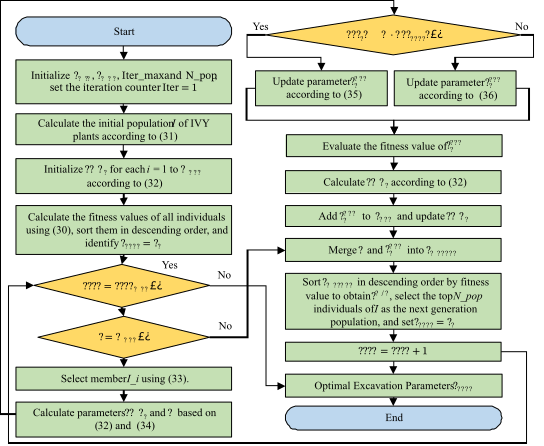
Based on the excavation trajectory optimization problem addressed in this study, the implementation process of the IVY algorithm is detailed as follows:
Parameter Initialization: Set the minimum value \(I_{\min}\), maximum value \(I_{\max}\), iteration count \(Iter_{\max}\), and population size \(N_{pop}\) for each variable. In this study, we set \(N_{pop}\) = 50, the number of optimization variables input to the trajectory optimization D = 8, and initialize the iteration counter \(Iter = 1\).
(2) Initial Population Generation: Calculate the initial population \(I = \left( I_{1},I_{2},...,I_{i},...,I_{N_{pop}} \right)\) of IVY plants according to (31).
| \[I_{i} = I_{\min} + rand(1,D) \odot \left( I_{\max} - I_{\min} \right),i = 1,\ldots,N_{pop}\] | (31) |
(3) Fitness Gap Calculation: Use (32) to compute the fitness gap \(\mathrm{\Delta}Gv_{i}\) for each individual, as well as the Hadamard product of two vectors, where \(i = 1,2,...,N_{pop}\).
| \[\Delta G_{vi} = \begin{cases} I_{i} \oslash \left( I_{\max} - I_{\min} \right), & \mathrm{Iter} = 1, \\ rand^{2} \odot \left( N(1,D) \odot \Delta G_{vi} \right), & \mathrm{Iter} > 1. \end{cases}\] | (32) |
(4) Iterative Optimization: Calculate the objective function value for all individuals in the initial population, sort them in descending order of fitness, and identify the optimal individual \(I_{best} = I_{1}\). Under the condition that the iteration count \(Iter \leq Iter_{\max}\), perform the following operations for each individual: Select individual \(I_{ii}\) from i = 1 to \(N_{pop}\) according to (33); then, compute \(\beta\) based on (34). If \(Q\left( I_{i} \right) < \beta \cdot f\left( I_{best} \right)\), update \(I_{i}^{new}\) using (35); otherwise, update it using (36). Here, Q represents the fitness function shown in (30). Finally, evaluate the fitness of \(I_{i}^{new}\) and calculate the new fitness gap; add \(I_{i}^{new}\) to the new population vector \(I_{new}\) and update \(\mathrm{\Delta}Gv_{i} = \mathrm{\Delta}Gv_{i}^{new}\).
| \[I_{ii} = \begin{cases} I_{j - 1}^{s}, & I_{i} = I_{j}^{s}, \\ I_{i}, & I_{i} = I_{Best}. \end{cases}\] | (33) |
| \[\beta = (2 + rand)/2\] | (34) |
| \[I_{i}^{new} = I_{i} + \left| N(1,D) \right| \odot \left( I_{ii} - I_{i} \right) + N(1,D) \odot \mathrm{\Delta}Gv_{i}\] | (35) |
| \[I_{i}^{new} = I_{best} \odot \left( rand(1,D) + N(1,D) \odot \mathrm{\Delta}Gv_{i} \right)\] | (36) |
(5) Population Update: Merge the original population I and the new population \(I_{new}\) to form a combined population \(I_{Merged}\). Sort \(I_{Merged}\) in descending order of fitness value, select the top \(N_{pop}\) individuals as the next generation population, and set \(I_{best} = I_{1}\).
(6) Iteration Counter Update: Increment the iteration counter: \(Iter = Iter + 1\).
(7) Termination Output: When the iteration ends, output the optimal solution \(I_{best}\) and the optimal variable set found by the IVY optimizer, thereby obtaining the optimal joint‑space trajectory parameters.
4. Experimental Verification and Result Analysis
4.1. Overview of Experiments
This chapter focuses on the core objective of engineering intelligence to enable autonomous decision‑making in loader excavation. It carries out an end‑to‑end experiment, spanning from virtual simulation verification to real‑world validation. The objective is to verify the effectiveness of the proposed trajectory optimization method, which combines an objective prediction and computation model with the IVY intelligent optimization algorithm. This integration ensures that the intelligent algorithm can generate optimal trajectories that satisfy engineering performance requirements under both simulated and real operating conditions. The experiment consists of two stages. In the first stage, it is conducted on the EDEM‑RecurDyn co‑simulation platform. By utilizing the material morphology data obtained from EDEM and the objective prediction model, the process performs trajectory optimization and multi‑algorithm comparisons to validate the superiority of the proposed method. The second stage extends to outdoor real‑world tests. It employs binocular vision to perceive actual material morphology, reuses the prediction model with adjusted variable ranges, and applies the IVY algorithm to generate the optimal joint‑space trajectory, which is then converted into the corresponding driving‑space trajectory, thereby verifying the practical feasibility of the proposed method.
4.2. Trajectory Optimization Validation in Simulation
4.2.1. Linear Trajectory Planning and Parameter Configuration
Based on the EDEM-RecurDyn platform, a loader excavation co-simulation environment was established, reusing the material model and loader multibody dynamics model from Section 2.3 to simulate a real excavation scenario. Following the method in Section 2.4.2, linear trajectory planning is performed in the world coordinate system. The specific procedure is as follows: First, based on the actual parameters of the loader bucket, the variation range of K is set from 1 to 600 mm, with \(L_{A'B'}\) constrained to a minimum of 200 mm and \(L_{A'C'}\) ranging from 200 to 800 mm. Then, candidate linear trajectories are generated with a step size of 5 mm, as shown in Fig. 14, yielding a feasible K value range of [189, 214] that satisfies the requirement of 80% to 110% of the rated bucket capacity, corresponding to 25 terminal positions and orientations. Finally, through inverse kinematic calculations on the feasible K range, the final admissible boom angle (\(\varphi_{1}\)) range is obtained as [‑38.8°, ‑36.6°], which provides variable boundaries for subsequent trajectory optimization.
Before employing the IVY algorithm for trajectory optimization, the value ranges and precision levels of each optimization variable are configured, as detailed in TABLE III. Among these, the range of \(\varphi_{1}\) is determined by the aforementioned linear trajectory planning. Furthermore, prior to evaluating fitness by generating task‑space trajectories through forward kinematics from the joint‑space curves produced by iteratively sampling the optimization variables, spline‑curve fitting is applied to the bucket‑tilting angle, boom angle, and vehicle‑speed curves. This ensures that the resulting trajectories are as smooth as possible, thereby reducing impact and wear on the machine structure.
TABLE III
Range and Precision Settings of Optimization Variables under Simulated Conditions
| Optimization Variable / Unit | Value Range | Precision |
| \(\text{t}_{\text{1}}\)/s | [2,5] | 0.1 |
| \(\text{t}_{2}\)/s | [2,5] | 0.1 |
| \(\text{t}_{3}\)/s | [2,5] | 0.1 |
| \(\text{t}_{4}\)/s | [2,5] | 0.1 |
| \(\text{t}_{5}\)/s | [0,5] | 0.1 |
| \(\text{t}_{6}\)/s | [3,5] | 0.1 |
| \(\text{v}_{\text{x1}}\)/mm | [100,200] | 1 |
| \(\text{φ}\)1/° | [-38.8,-36.6] | 0.1 |
4.2.2. Multi-Algorithm Comparative Validation
To evaluate the performance advantage of the IVY algorithm in trajectory optimization, two widely used algorithms in engineering applications—Particle Swarm Optimization (PSO) and Grey Wolf Optimizer (GWO)—were selected for comparison. To ensure a fair comparison, both the iteration count and population size were kept identical across all algorithms. The specific parameter settings are listed in TABLE IV, and all other parameters were set to their default initial values. In this study, the maximum number of iterations for the algorithm is uniformly set to 100, and the population size is set to 50. This parameter configuration is established with reference to extensive empirical studies on metaheuristic algorithms, achieving an optimal balance between optimization accuracy and computational cost [30,31].
TABLE IV
Parameter Settings of Different Algorithms
| Algorithm | IVY | PSO | GWO |
| Parameter Settings | epoch=100 pop_size=50 |
epoch=100 ; pop_size=50 c1=2.05 ; c2=2.05 w_min=0.4 ; w_max=0.9 |
epoch=100 pop_size=50 |
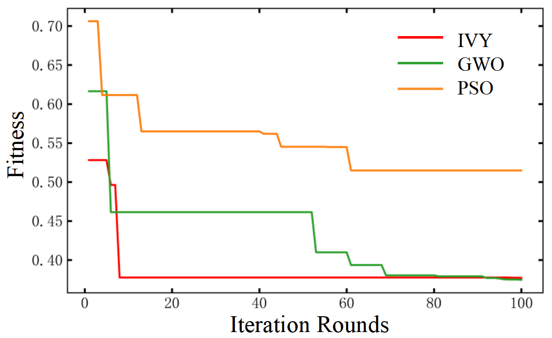
After 100 iterations, the variation curves of the optimization fitness values for the three algorithms are shown in Fig. 15. Analysis of the curves reveals the following: Since a lower fitness value indicates a better trajectory, the final fitness value of the IVY algorithm is approximately 26% lower than that of the GWO algorithm, meaning its fitness level is improved by approximately 26%, demonstrating superior optimization accuracy. Although the final fitness value of IVY is close to that of the PSO algorithm, its convergence speed is approximately 88% faster, confirming its superiority and feasibility for applications in this field.
4.2.3. Generation of Optimal Trajectories in Simulation
The optimized values of each variable obtained by the IVY algorithm when achieving the optimal fitness are listed in TABLE V. Visualizing these optimal variables yields the bucket‑tilting angle, boom angle, and vehicle speed curves, as shown in Fig. 16. The three curves exhibit excellent temporal coordination, with smooth action transitions and continuous, well‑connected trajectories. This effectively ensures operational fluidity, improves energy utilization efficiency, and reduces impact on the hydraulic system.
TABLE V
Optimal Parameters Obtained by the IVY Algorithm under Simulated Conditions
| Variable / Unit | Value | Variable / Unit | Value |
| \(\text{t}_{\text{1}}\)/s | 3.3 | \(\text{t}_{\text{5}}\)/s | 2.4 |
| \(\text{t}_{\text{2}}\)/s | 3.7 | \(\text{t}_{\text{6}}\)/s | 4.7 |
| \(\text{t}_{\text{3}}\)/s | 3.7 | \(\text{v}_{\text{x1}}\)/mm | 102.2 |
| \(\text{t}_{\text{4}}\)/s | 2.9 | \(\text{φ}\)1/° | -37.3 |
 |
|
| (a)Boom Angle Variation Curve | (b)Bucket‑Tilting Angle Variation Curve |
 |
|
(c)Vehicle Speed Variation Curve |
|
Fig. 16. Optimal Joint‑Space Curves and Vehicle Speed Curve under Simulated Conditions
4.3. Trajectory Optimization Application in Real-World Conditions
Based on the optimal algorithm and model validated through simulation in Section 3.2, this section conducts validation under real-world working conditions. It should be noted that the objective of field validation differs from that of the simulation stage: the simulation stage has already demonstrated the theoretical superiority of the IVY algorithm through quantitative comparison, while this section focuses on validating the feasibility of engineering implementation, aiming to achieve a complete technical loop from simulation to physical application.
4.3.1. Real-World Experimental Setup
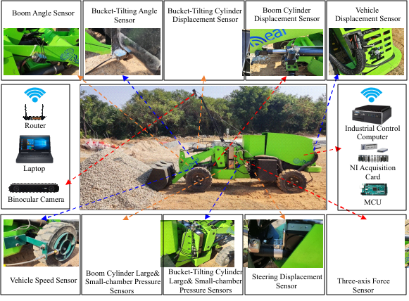
To achieve the goal of translating simulation into practice, an experimental system for loader excavation trajectory optimization is established. The field setup is illustrated in Fig. 17, which includes a 1:4‑scale loader prototype, a binocular vision perception module, an NI data acquisition system, and other components. The experimental procedure is designed as follows:
(1) Data Acquisition: Displacement, angle, and pressure sensors are used to synchronously collect mechanical state information during excavation, providing measured data for trajectory validation.
(2) Morphology Perception: Binocular vision replaces the method of directly exporting material data from EDEM in simulations, enabling non‑contact, accurate perception of the real material‑pile morphology.
(3) Trajectory Optimization and Transformation: The host computer deploys the IVY algorithm and the optimization‑objective prediction model. After completing trajectory optimization, the optimal joint‑space trajectory is converted into a driving‑space trajectory via inverse kinematics, thereby providing input commands for intelligent control.
4.3.2. Binocular Vision-Based 3D Reconstruction of Material Surface
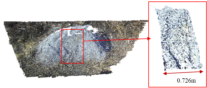
Unlike simulations where data can be directly exported from software, real‑world conditions require obtaining morphological information through perception devices, typically using cameras [32] or LiDAR [33]. This study employs a low‑cost binocular camera (mounted on the loader's front frame via a bracket) to achieve 3D reconstruction of the material pile. The specific procedure is as follows:
(1) Image Acquisition and Pre‑processing: As the loader approaches the material pile, the binocular camera captures left‑ and right‑view images of the pile. Through feature point detection and matching, disparity calculation, and depth map generation, 3D point cloud data is ultimately produced.
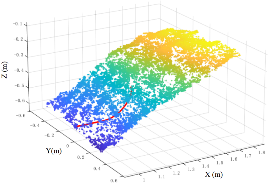
(2) Region of Effective Cropping: Based on the bucket width, the effective region of the material pile point cloud is cropped, as shown in Fig. 18, to reduce subsequent computational load and improve processing efficiency.
(3) Material Pile Surface Fitting: The point cloud within the effective region undergoes a two‑step fitting process: First, a first‑order fitting is applied to obtain the angle of repose of the material pile, as shown in Fig. 19(a). This is used for initial linear trajectory planning to determine key points of the bucket‑tip trajectory. Second, a polynomial fitting is performed to derive a high‑precision surface shape of the material pile, as illustrated in Fig. 19(b), ensuring the accuracy of excavation‑volume calculations.
(4) Coordinate System Unification: Since the coordinate system of the binocular camera differs from that of the loader kinematic model, coordinate transformation is necessary to ensure proper alignment between the trajectory and the material position, thereby avoiding computational errors. According to Section 2.2, the base point \(O_{0}(X_{0},Y_{0})\) of the kinematic model is located at the hinge point between the boom and the front frame of the vehicle. Given the camera coordinates as \(O_{camera}(X_{camera},Y_{camera})\), the coordinate systems are unified using (37).
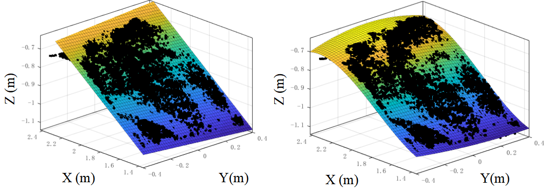 |
|
| (a)First-order Fitting | (b)polynomial fitting |
Fig. 19. Material Surface Fitted by First-order and Polynomial Methods
| \[\text{T}_{{\text{O}_{\text{0}}\text{→}\text{O}}_{\text{camera}}} = \begin{bmatrix} \text{R} & \text{T}_{\text{P}} \\ \text{0} & \text{1} \end{bmatrix} = \begin{bmatrix} \text{cos(}\text{θ}\text{)} & \text{-sin(}\text{θ}\text{)} & \begin{matrix} \text{0} & \text{∆}\text{x} \end{matrix} \\ \text{sin(}\text{θ}\text{)} & \text{cos(}\text{θ}\text{)} & \begin{matrix} \text{0} & \text{∆}\text{y} \end{matrix} \\ \begin{matrix} \text{0} \\ \text{0} \end{matrix} & \begin{matrix} \text{0} \\ \text{0} \end{matrix} & \begin{matrix} \begin{matrix} \text{1} & \text{∆}\text{z} \end{matrix} \\ \begin{matrix} \text{0} & \text{1} \end{matrix} \end{matrix} \end{bmatrix}\] | (37) |
In the equation, R is the rotation matrix, \(T_{P}\)is the translation matrix, \(\theta\) is the installation tilt angle of the binocular camera rotated around the axis parallel to the Y‑axis relative to the positive X‑axis direction, and \(\mathrm{\Delta}x\), \(\mathrm{\Delta}y\), and \(\mathrm{\Delta}z\) are the coordinate differences of the two coordinate system origins in the horizontal, lateral, and vertical directions, respectively. Through on‑site installation measurements, it is determined that \(\theta\) = 60, \(\mathrm{\Delta}x\) = 30, \(\mathrm{\Delta}y = 0\), \(\mathrm{\Delta}z = 854\ mm\).
After coordinate unification, the superimposed display of the material point cloud and the kinematic model is shown in Fig. 20.
4.3.3. Optimal Trajectory Generation and Transformation in Real-World Conditions
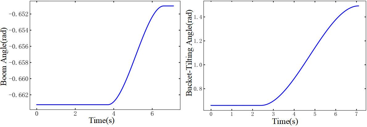
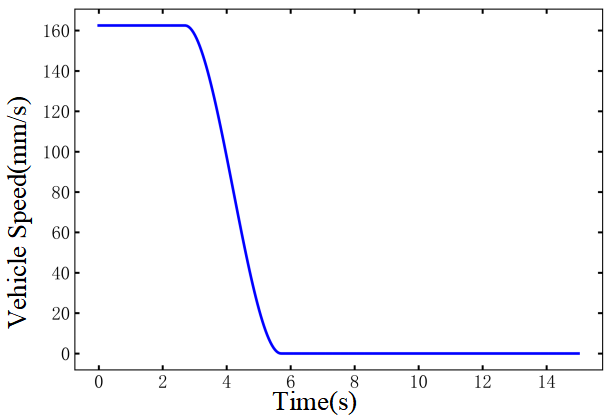
Since the simulation model simplifies factors such as air resistance and mechanical vibration, and reduces computational load through simplified contact models, while actual working conditions involve physical hardware and real‑time feedback that introduce additional time overhead, and delays in hydraulic system and motor execution extend excavation time, the optimization variable ranges are readjusted to match the physical constraints of the actual vehicle. The IVY algorithm is then used to re‑optimize the trajectory. The resulting optimal parameters are listed in TABLE VI, and the corresponding optimal joint‑space curves and vehicle speed curve are shown in Fig. 21.
TABLE VI
Optimal Trajectory Parameters under Actual Working Conditions
| Variable / Unit | Value Range | Optimized Value |
| \(\text{t}_{\text{1}}\)/s | [1,10] | 2.7 |
| \(\text{t}_{2}\)/s | [1,10] | 3.0 |
| \(\text{t}_{3}\)/s | [1,10] | 1.3 |
| \(\text{t}_{4}\)/s | [1,10] | 6.0 |
| \(\text{t}_{5}\)/s | [1,10] | 7.0 |
| \(\text{t}_{6}\)/s | [1,10] | 8.0 |
| \(\text{v}_{\text{x1}}\)/mm | [100,200] | 162.5 |
| \(\text{φ}\)1/° | [-34.7,-32.9] | -32.9 |
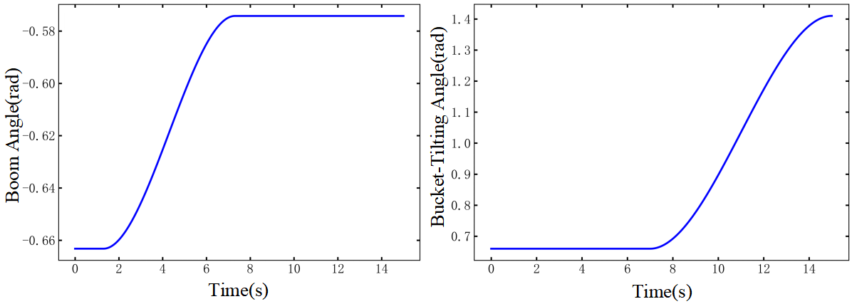 |
|
| (a)Boom Angle Variation Curve | (b)Bucket‑Tilting Angle Variation Curve |
 |
|
(c)Vehicle Speed Variation Curve |
|
Fig. 21. Optimal Joint‑Space Curves and Vehicle Speed Curve under Actual Working Conditions
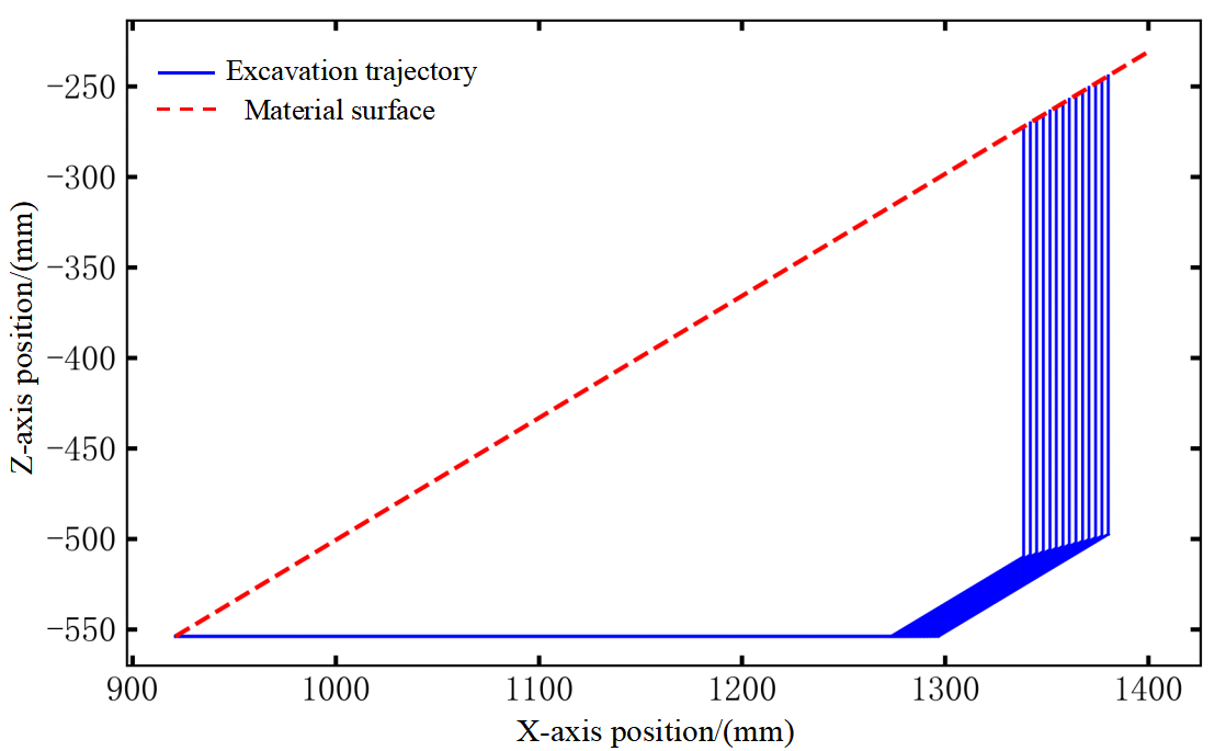
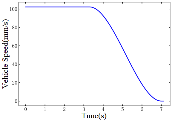
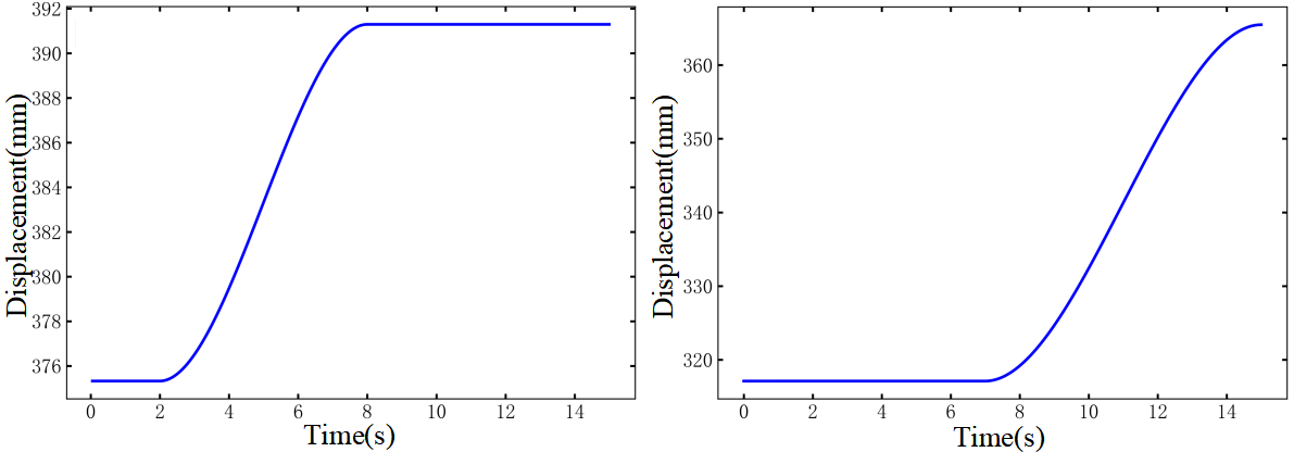
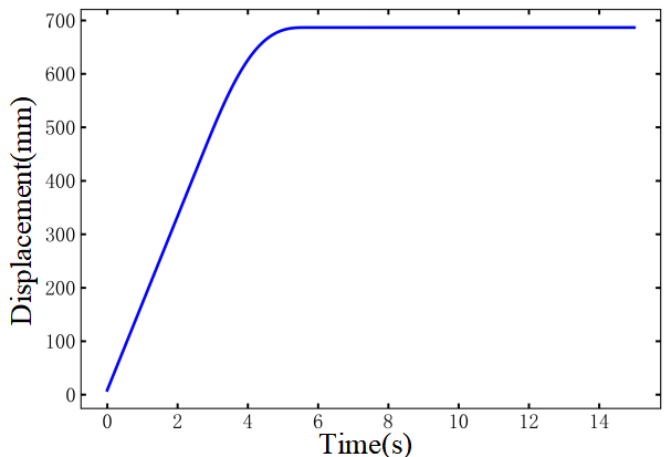
Through inverse kinematics inference, the optimal trajectory in joint space is transformed into the optimal trajectory in driving space, as shown in Fig. 22. This trajectory can be directly used as input commands for intelligent control, enabling efficient and autonomous excavation operation of the loader via trajectory tracking.
 |
|
| (a)Lift Cylinder Displacement Variation Curve | (b)Bucket‑Tilting Cylinder Displacement Variation Curve |
 |
|
(c)Vehicle Displacement Variation Curve |
|
Fig. 22. Optimal Driving‑Space Curves under Actual Working Conditions
5. Conclusion
5.1. Main Conclusions
This research addresses the limitations of purely data-driven approaches (characterized by high data dependency and significant labeling costs) and purely model-driven methods (suffering from weak generalization and limited fidelity to real-world conditions). A bidirectional data-model synergistic framework is established, providing an efficient and cost-effective solution for intelligent construction machinery operation. This work demonstrates the potential of deeply integrating artificial intelligence technology with industrial applications. The core conclusions are as follows:
(1) An optimization objective prediction method based on EDEM-RecurDyn co-simulation is proposed. A high-fidelity material-machine interaction model is constructed through coupled simulation to efficiently obtain resistance data for multiple trajectories. These data, integrated with a CNN-GRU model, enable accurate prediction of optimization objectives. This approach avoids reliance on massive real-world measurement data required by purely data-driven methods while enhancing engineering applicability and significantly reducing data acquisition and modeling costs.
(2) An intelligent optimization strategy based on the IVY algorithm is proposed. Compared with conventional algorithms such as PSO and GWO, the proposed method achieves faster convergence, higher optimization quality, and efficiently generates smooth, adaptive excavation trajectories. This provides an effective optimization paradigm for AI-based trajectory optimization in construction machinery applications.
(3) A hybrid data-model-driven trajectory optimization system is constructed. By integrating prior knowledge with simulated and measured data, the system ensures theoretical accuracy while enhancing practical applicability. The successful transition from simulation validation to real-world application provides a new approach for intelligent trajectory optimization of construction machinery, overcoming the limitations of single-mode-driven methods.
5.2. Future Work
Due to experimental constraints, the optimal trajectories have not yet been deployed for validation on physical machines. Future research will focus on deepening the integration of AI with industrial applications to enhance the universality and intelligent capabilities of the proposed technology:
(1) Develop intelligent control algorithms suitable for complex equipment such as loaders, deploy the optimized trajectories on physical machines, and compare them with manually operated trajectories to validate the effectiveness of the proposed method.
(2) Integrate reinforcement learning and online decision-making algorithms to enable real-time dynamic adjustment of excavation trajectories. Further explore intelligent scheduling strategies for multi-machine collaborative operations, advancing the application of AI technology in higher-level industrial scenarios such as construction machinery fleet operations.
(3) Construct a model library of material piles with various material types and angles of repose, along with an excavation information database. Integrate these resources with transfer learning techniques to achieve rapid cross-scenario trajectory adaptation, thereby enhancing the industrial universality of the solution.
Acknowledgment
The work presented in this paper has been supported by National Natural Science Foundation of China (51905460), Natural Science Foundation Program of Fujian(2022J01060), and National Key R&D Program of China (2020YFB1709904, 2020YFB1709901)
Declarations
The authors declare that they do not have any commercial or associative interest that represents a conflict of interest in connection with the work submitted
References
- S. Dadhich, U. Bodin, and U. Andersson, “Key challenges in automation of earth-moving machines,” Autom. Constr., vol. 68, pp. 212–222, Aug. 2016, doi: 10.1016/j.autcon.2016.05.009.
- S. Dadhich, “Automation of wheel-loaders,” Licentiate thesis, Dept. Comput. Sci. Elect. Space Eng., Luleå Univ. of Technol., Luleå, Sweden, 2018.
- Y. Fang, J. Hu, W. Liu, et al., “Smooth and time-optimal S-curve trajectory planning for automated robots and machines,” Mech. Mach. Theory, vol. 137, pp. 127–153, Jul. 2019, doi: 10.1016/j.mechmachtheory.2019.03.019.
- S. Wang, Y. Wu, L. Hou, and Z. Yang, “Predictive modeling for soft measurement of loader driveshaft torque based on large-scale distributed data,” Measurement, vol. 210, Mar. 2023, Art. no. 112566, doi: 10.1016/j.measurement.2023.112566.
- B. Frank, J. Kleinert, and R. Filla, “Optimal control of wheel loader actuators in gravel applications,” Autom. Constr., vol. 91, pp. 1–14, Jul. 2018, doi: 10.1016/j.autcon.2018.03.005.
- J. Yao et al., “Bucket loading trajectory optimization for the automated wheel loader,” IEEE Trans. Veh. Technol., vol. 72, no. 6, pp. 6948–6958, Jun. 2023, doi: 10.1109/TVT.2023.3236507.
- T. Zhang, T. Fu, X. Song, and F. Qu, “Multi-objective excavation trajectory optimization for unmanned electric shovels based on pseudospectral method,” Autom. Constr., vol. 136, Apr. 2022, Art. no. 104176, doi: 10.1016/j.autcon.2022.104176.
- Y. Chen, G. Shi, C. Tan, and Z. Wang, “Machine learning-based shoveling trajectory optimization of wheel loader for fuel consumption reduction,” Appl. Sci., vol. 13, no. 13, Jun. 2023, Art. no. 7659, doi: 10.3390/app13137659.
- I. P. Timofeev and A. Y. Kuzkin, “PNB type loader shoveling arm motion irregularity in dependence of its mass,” J. Min. Inst., vol. 221, pp. 717–723, Oct. 2016, doi: 10.18454/pmi.2016.5.717.
- X. Tan et al., “Reinforcement learning-based trajectory planning for continuous digging of excavator working devices in trenching tasks,” Comput.-Aided Civ. Infrastruct. Eng., vol. 40, no. 13, pp. 1847–1870, Jan. 2025, doi: 10.1111/mice.13428
- Z. Huai,Y. Chen Y, Q. Hong, “Optimizing of autonomous loading trajectory of loader based on various interpolation methods,” Min. Process. Equip., vol. 50, no. 2, pp. 10–15, Feb. 2022, doi: 10.16816/j.cnki.ksjx.2022.02.012. (in Chinese)
- T. Zhou, B. Chen, Y. Chen, Y. He, and C. Wang, “Data-driven optimization method for automatic shoveling trajectory of loaders,” in Proc. ICAMTMS 2023, Dalian, China, 2023, pp. 257–262.
- T. Zhang, T. Fu, T. Ni, H. Yue, Y. Wang, and X. Song, “Data-driven excavation trajectory planning for unmanned mining excavator,” Autom. Constr., vol. 162, Jun. 2024, Art. no. 105395, doi: 10.1016/j.autcon.2024.105395.
- S. Dadhich, F. Sandin, U. Bodin, and S. Sandin, “Adaptation of a wheel loader automatic bucket filling neural network using reinforcement learning,” in Proc. IJCNN, Glasgow, UK, 2020, pp. 1–9.
- S. Li, X. Zhou, S. Wang, Y. Pan, T. Guo, and L. Hou, “Excavation trajectory planning based on feedforward neural network and physics-encoded optimization,” Autom. Constr., vol. 181, Jan. 2026, Art. no. 106634, doi: 10.1016/j.autcon.2025.106634.
- Y. Meng, H. Fang, G. Liang, and R. Luo, “Optimization of the shoveling trajectory of an LHD loader based on a discrete element method and experiment,” Energies, vol. 12, no. 20, Oct. 2019, Art. no. 3919, doi: 10.3390/en12203919.
- X. Yu, Y. Huai, X. Li, et al, “Shoveling trajectory planning method for wheel loader based on kriging and particle swarm optimization,” J. Jilin Univ. (Eng. Technol. Ed.), vol. 50, no. 2, pp. 54–61, Mar. 2020, doi: 10.13229/j.cnki.jdxbgxb20190766.(in Chinese)
- Q. Zhao, L. Gao, D. Wu, et al., “E-GCDT: Advanced reinforcement learning with GAN-enhanced data for continuous excavation system,” Appl. Intell., vol. 55, no. 6, pp. 1–22, Feb. 2025, doi: 10.1007/s10489-025-06308-5.
- S. Wang, J. Huang, L. Hou, Y.Wu, “Resistance prediction technology of loader shoveling operation based on incremental learning,” Electro-Mech. Eng., vol. 40, no. 5, pp. 28–36, May 2024, doi: 10.19659/j.issn.1008–5300.2024.05.005. (in Chinese)
- S. Wang, S. Yu, L. Hou, H. Fang, Y. Meng, and S. Li, “Prediction of bucket fill factor of loader based on three-dimensional information of material surface,” Electronics, vol. 11, no. 18, Sep. 2022, Art. no. 2841, doi: 10.3390/electronics11182841.
- B. Wu, L. Hou, S. Wang, Y. Yin, and S. Yu, “Predictive modeling of loader's working resistance measurement based on multi-sourced parameter data,” Autom. Constr., vol. 149, May 2023, Art. no. 104805, doi: 10.1016/j.autcon.2023.104805.
- R. Filla and B. Frank, “Towards finding the optimal bucket filling strategy through simulation,” in Proc. 15th Scandinavian Int. Conf. Fluid Power (SICFP), Linköping, Sweden, 2017, pp. 393–401.
- Y. Chen, Y. Meng, S. Xiang, et al, “Shovel path planning of loader based on beetle antennae search,” Comput. Integr. Manuf. Syst., vol. 29, no. 7, pp. 2201–2214, Jul. 2023, doi: 10.13196/j.cims.2023.07.006.(in Chinese)
- B. Wu, S. Wang, L. Hou, Y. Yin, and S. Yu, “Fast estimation of loader’s shovel load volume by 3D reconstruction of material piles,” Chin. J. Mech. Eng., vol. 36, no. 1, Oct. 2023, Art. no. 117, doi: 10.1186/s10033-023-00945-y.
- S. Wang, Y. Yin, Y. Wu, L. Hou, H. Fang, and Y. Meng, “Modeling and verification of an acquisition strategy for wheel loader’s working trajectories and resistance,” Sensors, vol. 22, no. 16, Aug. 2022, Art. no. 5993, doi: 10.3390/s22165993.
- S. Wang, S. Huang, L. Hou, Y. Meng, H. Fang, and S. Li, “Research on predictive modeling method of loader working resistance in a sensor-less environment,” Eng. Appl. Artif. Intell., vol. 138, Dec. 2024, Art. no. 109263, doi: 10.1016/j.engappai.2024.109263.
- H. Feng, J. Jiang, N. Ding, S. Ma, and J. Zhou, “Multi-objective time-energy-impact optimization for robotic excavator trajectory planning,” Autom. Constr., vol. 156, Dec. 2023, Art. no. 105094, doi: 10.1016/j.autcon.2023.105094.
- J. Tang, G. Liu, and Q. Pan, “A review on representative swarm intelligence algorithms for solving optimization problems: Applications and trends,” IEEE/CAA J. Autom. Sinica, vol. 8, no. 10, pp. 1627–1643, Oct. 2021, doi: 10.1109/JAS.2021.1004129.
- M. Ghasemi, M. Zare, P. Trojovský, E. Akbari, and A. Ghasemi, “Optimization based on the smart behavior of plants with its engineering applications: Ivy algorithm,” Knowl.-Based Syst., vol. 295, Jul. 2024, Art. no. 111850, doi: 10.1016/j.knosys.2024.111850.
- S. Vadi, M. Bildirici, and O. Kaplan, “Performance Comparison of Metaheuristic and Hybrid Algorithms Used for Energy Cost Minimization in a Solar–Wind–Battery Microgrid,” Sustainability, vol. 17, no. 19, pp. 8849, 2025.
- D. Kumar, Y. K. Chauhan, and A. S. Pandey, “Performance Investigation of Renewable Energy Integration in Energy Management Systems with Quantum-Inspired Multiverse Optimization,” Sustainability, vol. 17, no. 8, pp. 3734, 2025.
- Y. Zhang, F. Yang, H. Yuan, S. Li, and X. Song, “3D reconstruction of coal pile based on visual scanning of bridge crane,” Measurement, vol. 242, Jan. 2025, Art. no. 116146, doi: 10.1016/j.measurement.2024.116146.
- G. Chen, Y. Wang, X. Li, Q. Bi, and X. Li, “Shovel point optimization for unmanned loader based on pile reconstruction,” Comput.-Aided Civil Inf., vol. 39, no. 14, pp. 2187–2203, Oct. 2024, doi: 10.1111/mice.13190.